Solving Threading with the Producer Consumer Model

Introduction

You’ve rented out one of the larger EC2 instances to do some batch processing on, but it can still take for-ev-er for some particular jobs to finish up. We can see that we’re only using one of the virtual cores that come with it; the remaining three or seven are staying idle. Threading the application seems like a great way to speed up the processing by leveraging the remaining cores. However, how to best split up the work is still an issue. If you assume that all the work takes a uniform amount of time, it’s easy to split to give each thread an equal number of tasks. In the real world, though, it’s rare that all tasks are uniform. For example, say you added 10 new fields to a form after the first 10,000, and another 20 fields after the first 40,000. The thread assigned the first 10,000 or so are going to finish much quicker than the remaining ones. They could grab a random form, but where does the master list reside? How will they know which thread has gotten which piece of information?

This is a class of problems known as the Producer – Consumer problem. In the most general terms, N threads are listening for data that’s coming from one particular source. In operating systems, this can be input listeners, network, etc. For our uses here, we’ll have one producer thread passing on information to N number of workers.

For this problem, we’ll use an easy example of downloading web pages for a load test. We’ll attempt to download 50 pages per second spread out accross 16 threads. Since these are heavy on IO wait, we can run more threads than there are processors on the machine. The producer will update a shared memory location, and all the consumers will retrieve one entry at a time from the data structure. In this way, we can be sure that each thread is only doing work if it has no other work to do, so it’ll be evenly distributed across all workers.

Implementation

Shared Memory

This is the tie that binds the producer and the consumer together. In short, the shared memory structure allows the producer thread a place to store tasks that workers can grab whenever they determine they need more work to do. All the methods in this class are synchronized to avoid the dreaded ConcurrentModificationException. Since threads can preempt other threads, there’s no guarantee that a List.remove() method will finish before another thread tries to call List.remove() again, which can result in some corrupted data structures.

public class SharedDataStructure {
    //Data structure to store the urls
    protected static final List<String> urls;
    static {
        urls = new LinkedList<String>();
    }
    
    //The producer should call this method when it wants to add another url to be downloaded
    public static void push(String url) {
        synchronized(urls) {
            urls.add(url);
        }
    }
    
    // The consumers should call this to get another url to download
    public static String pop() {
        synchronized(urls) {
            if (urls.size() > 0) {
                return urls.remove(0);
            }
            return null;
        }
    }
}

Producer

The producer in this case is just going to grab 50 random pages from a static list of webpages to be included in the test. In an ideal test, these should be weighted according to the access patterns of the website, but we’re going simple here!

public class Producer extends Thread {
    private static final String[] webpages = { "http://google.com", "http://bing.com", "http://yahoo.com", "http://reddit.com" };

    @Override
    public void run() {
        Random random = new Random();
        while (true) {
            for (int i = 0; i < 50; i++) {
                String url = webpages[random.nextInt(webpages.length])];
                SharedDataStructure.push(url);
            }
            try {
                sleep(1000);
            } catch (InterruptedException e) {
                e.printStackTrace();
            }
        }
    }
}

Consumer

The sole functions of the consumer are to read the next value off of the shared memory structure and grabbing the web page. In this example, I’m just going to read the first line from the response to keep the code short; in practice, this should also be sufficient for certain types of load tests, though you’ll probably always want to download the whole page.

public class Consumer extends Thread {
    @Override
    public void run() {
        while (true) {
            String url = SharedDataStructure.pop();
            if (url != null) {
                try {
                    URLConnection urlConnection = new URL(url).openConnection();
                    InputStreamReader reader = new InputStreamReader(urlConnection.getInputStream());
                    reader.read();
                } catch (IOException e) {
                    e.printStackTrace();
                }
            } else {
                try {
                    sleep(10);
                } catch (InterruptedException e) {
                    e.printStackTrace();
                }
            }
        }
    }
}

Starting it up

Now that we’ve got all three parts of the program written, let’s start it up!

public class Main {
    public static void main(String args[]) {
        for (int i = 0; i < 16; i++) {
            new Consumer().start();
        }
        new Producer().start();
    }
}

Conclusion

As we’ve discovered here, generalizing threaded batch processes to producer consumer type problems allows us to easily divide work fairly among as many threads as we’d like!

If you’d like to read further about the this, the following books are a great place to start for beginners and intermediate programmers!

Using Maps for ETL Aggregation

Introduction

You’re trying to decide which products are most important to your customers, or maybe the marketing team is interested in how many widgets have been sold to each industry, or you’re trying to list which five pages in your project are most viewed. To add another wrinkle, the key stakeholders in your project want to be able to interact with the information themselves, and you’d happy they won’t keep coming to you every time they need a data pull.

The key question still remains, how do you aggregate all this information over millions of records in a reasonable amount of time? The the previous part of this tutorial, we covered how to use sets for duplicate information, and there is a way to make that work here. However, we’d prefer something a little cleaner.

In this tutorial, we’ll talk about using maps to efficiently handle aggregations across multiple tables, so you’re left with one insert per unit instead of tons of updates to records in the database. Or, worse still, millions of queries

Getting Started

What are Maps?

The quick answer is that maps are data structures that contain a set of key value pairs. One key maps to exactly one value in the dataset. For example, in the following example:

Key1=Value1

Key2=Value2

Key3=Value3

Key1=Value4

The final value of the data set will be (Key1=Value4, Key2=Value2, Key3=Value3). These are similar to associative arrays found in JavaScript and in PHP.

The reason why we’re using hash maps here are for their insert / index speed. In a typical list, accessing an individual element is time O(N), adding to it is O(1). What we’d find then is that querying a list for its values across all keys would result in a runtime of O(N2), whereas maps would be a runtime of O(N) – iterating over all keys. For small sets, this difference is pretty negligible, but it quickly becomes an issue when we start getting into the millions of records. Suddenly, you need quadrillions of operations for lists instead of millions for maps.

Example database

For this example, Discogs.com is nice enough to give away their entire data set once of month full of of musicians, albums, labels, etc, so we’ll be using a much, much simplified version of their amazing database. For this example, we’re interested in collecting aggregate information about a particular artist to determine the breadth of their music industry exposure.

Screen Shot 2016-01-30 at 9.15.05 PM

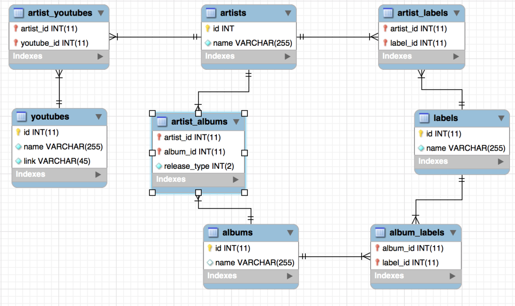
Above is a MySQL workbench screenshot describing how all this information fits together in our database. This does violate 2NF, but it’s useful to see the relationship between all the elements in the dataset. Artists (middle top) contains a globally unique id as well as the artists’ names. We also have labels (center right), albums, (middle bottom) and youtube videos (center left). These are connected through their various join tables – artist_albums, artist_labels, album_labels, and artist_youtubes. On important note is that artist_albums also contains a field, release_type, which determines if this was their release, if they guess stared on the album, if they produced it, etc.

Implementation


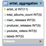
Screen Shot 2016-01-30 at 9.22.20 PM

We’ll be populating a table that contains the following entries:

  • total_albums_count – the number of albums the artist is associated with
  • main_releases – the number of albums this artist has released
  • appeared_on_releases – the number of albums this artist had a contributing vocal role on (backup singer, guest rapper, etc.)
  • producer_releases – the number of albums this artist was a producer on
  • youtubue_videos – the number of youtube videos we found for this artist
  • labels – the number of labels this artist has appeared on

So the first thing we’ll do is create a Java class to hold this information

public class ArtistAggregation {
	private int artistId;
	private int mainReleases;
	private int appearedOnReleases;
	private int producerReleases;
	private int youtubeVideos;
	private int labels;
	public int getArtistId() {
		return artistId;
	}
	public void setArtistId(int artistId) {
		this.artistId = artistId;
	}
	public int getMainReleases() {
		return mainReleases;
	}
	public void setMainReleases(int mainReleases) {
		this.mainReleases = mainReleases;
	}
	public int getAppearedOnReleases() {
		return appearedOnReleases;
	}
	public void setAppearedOnReleases(int appearedOnReleases) {
		this.appearedOnReleases = appearedOnReleases;
	}
	public int getProducerReleases() {
		return producerReleases;
	}
	public void setProducerReleases(int producerReleases) {
		this.producerReleases = producerReleases;
	}
	public int getYoutubeVideos() {
		return youtubeVideos;
	}
	public void setYoutubeVideos(int youtubeVideos) {
		this.youtubeVideos = youtubeVideos;
	}
	public int getLabels() {
		return labels;
	}
	public void setLabels(int labels) {
		this.labels = labels;
	}
}


Putting it All Together

Now, let’s get into the meat of the article, how to use maps. What we’re going to do here is create a new map for every type of information and then combine into a composite data structure before inserting into the database. For this example, each map is going to be populated from one method that takes a query string with a specific structure as an argument. We’ll then iterate over the total set of all artist ids and check for the required information in the map to construct our final database object. If this sounds a little confusing, check out the code block below, and it’ll become a lot clearer.

We could do all of this on the fly using a visitor pattern for all of the methods that populate the map, but I generally shy away from that pattern. Over the life of the program, it doesn’t save us that much time or space, and it can be confusing to maintain for very large aggregation tables (think 50+ elements).

The following is exactly how this is all going to be implemented in Java:

// return a map with a key of the artist id and a value of whatever we're counting.
// The user must specify a query of the type "select artist.id, count(*) c from..."
private Map<Integer, Integer> fetchIdCount(Connection conn, String query) {
	Map<Integer, Integer> map = new HashMap<Integer, Integer>();
	Statement statement = conn.createStatement();
	ResultSet set = statement.executeQuery(query);
	while (set.next()) {
		map.put(set.getInt("id"), set.getInt("c"));
	}
	set.close();
	statement.close();
	return retval;
}

// Get all artist ids. We'll use this to iterate over later
private Set<Integer> fetchAllArtistIds(Connection conn) {
	Set<Integer> set = new HashSet<Integer>();
	Statement statement = conn.createStatement();
	ResultSet set = conn.createStatement("select id from artists");
	while (set.next()) {
		set.add(set.getInt("id"));
	}
	set.close();
	statement.close();
	return retval;
}

public Set<ArtistAggregation> aggregate(Connection conn) {
	Set<ArtistAggregation> retval = new HashSet<ArtistAggregation>();
	
	Set<Integer> allIds = fetchAllArtistIds(conn);
	Map<Integer, Integer> youtubes = fetchIdCount("select a.id, count(*) c from artists a, artist_youtubes ay where a.id=ay.artist_id group by a.id");
	//Assume the album_type code for producer is '5'
	Map<Integer, Integer> produced = fetchIdCount("select a.id, count(*) c from artists a, artist_albums aa where a.id=aa.artist_id and aa.release_type=5 group by a.id");
	//Assume the album_type code for appeared on is '2'
	Map<Integer, Integer> appearedOn = fetchIdCount("select a.id, count(*) c from artists a, artist_albums aa where a.id=aa.artist_id and aa.release_type=2 group by a.id");
	//Assume the album_type code for main release is '0'
	Map<Integer, Integer> mainRelease = fetchIdCount("select a.id, count(*) c from artists a, artist_albums aa where a.id=aa.artist_id and aa.release_type=0 group by a.id");
	Map<Integer, Integer> labels = fetchIdCount("select a.id, count(*) c from artists a, artist_labels al where a.id=al.artist_id group by a.id");
	
	for (Integer artistId : allIds) {
		ArtistAggregation aa = new ArtistAggregation(artistId);
		if (youtubes.contains(artistId)) {
			aa.setYoutubeVideos(youtubes.get(artistId));
		}
		if (produced.contains(artistId)) {
			aa.setProducerReleases(produced.get(artistId));
		}
		if (appearedOn.contains(artistId)) {
			aa.setAppearedOnReleases(appearedOn.get(artistId));
		}
		if (mainRelease.contains(artistId)) {
			aa.setMainReleases(mainRelease.get(artistId));
		}
		if (labels.contains(artistId)) {
			aa.setLabels(labels.get(artistId));
		}
	}
	
	return retval;
}

As you can see above, we’re first grabbing all the known artist ids and using that as a basis to determine if that artist does have entries into the various aggregation hash maps.

Conclusion

We’ve walked through why exactly you should use hash maps to store various pieces of aggregate information in order to construct the final object, and we’ve looked at how that type of system would work.

We can see from the above examples that this approach is simple, clean, and effective. Instead of querying the database N times (where N is the number of artists), we’re querying the database only one time for each type of aggregation, which results in execution speeds orders of magnitude quicker than the alternative!

Using Sets to Handle Duplication in Large Scale ETLs

Introduction

We’ve all been in the situation where you’re processing a ton of information for your ETLs, but you’re dealing with a lot of duplicates in the data. There are so many duplicates that you’re actually running out of memory or your database updates are taking forever. Ho do you deal with them? Do you throw all the entries into a list or an array and check to see if it’s been updated? That gets really expensive really fast as you iterate. Do you check against your database to see if it’s already been inserted? As you can probably guess, this takes for-ev-er. So what’s an alternative? Using Sets.

Implementation

For this blog entry, we’re going to take a pretty simple example of finding unique words in customer success emails. We later want to perform some sentiment analysis on these words to see how our customers perception of us is changing over time. Is this example contrived? Sure, but these principles are pretty easily extendable to any similar issues you might be facing.

What is a set?

A set is a simple data structure that can contain only one distinct value. For example, if we have an array of integers – [1,2,3,3,3,3,4,5,5,6] – and add it to a set, the result will be a data structure containing the values – [1,2,3,4,5,6]. If we have an array of strings – [‘what’, ‘the’, ‘what’, ‘said’, ‘liz’, ‘lemon’] – the result will be a data structure containing – [‘what’,’the’,’said’,’liz’,’lemon’]

Set’s are also notable in that they are constant time – O(1) – for inserts, deletions, and lookups. Lists… lists technically have an O(N) for inserts, but, practically speaking, doubly linked lists (LinkedList in Java) are constant time for appending to the end of the list. Array lists (ArrayList in Java) have an O(N) insert time if the underlying array needs to be resized. LinkedLists are O(N) for lookups and deletions, and ArrayLists are O(1) for lookup by index and O(N) for lookup by object; ArrayLists are also O(N) for deletions.

Given the running time of these algorithms, you can see that checking for duplicates for each value we’re processing is going to be a O(N2), but checking for duplicates in Sets for each value we’re processing is going to be a O(N) algorithm. In other words, checking for 1 million duplicates as their added in Lists is going to require 1 trillion operations; contrasting that with a Set, checking for 1 million duplicates as their added will only require 1 million operations.

Coding it out in Java

This is fine for simple data types, but in Java objects are given a name at construction time, something like “object-12′ or ‘object-521’ which is used as it’s hash entry. These strings are guaranteed to be unique, and they are what Java uses by default for determining a key into the set. So how do we get around this?

Internally, every Object in Java has two methods, hashCode() and equals(Object o) that must be overridden before the Set will know how to handle the object correctly. When adding, getting, or removing an entry from the Set, Java will first check to see if there’s a matching entry with the same hashCode() value. If so, it will then check to see if the two values are equal. In practice, it’s unlikely that there will be a hashCode() collision, so the equals function is mostly there as a safeguard just in case.

The class for the customer success word will look like the following:


public class CustomerSuccessWord {
	private int successId;
	private String word;
	private int hashCode;

	public CustomerSuccessWord(int successId, String word) {
		this.successId = successId;
		this.word = word;
		this.hashCode = (successId + "\t" + word).hashCode();
	}

	@Override
	public int hashCode() {
		return this.hashCode;
	}

	@Override
	public boolean equals(Object o) {
		boolean retval = false;
		if (o instanceof CustomerSuccessWord) {
			CustomerSuccessWord csw = (CustomerSuccessWord) o;
			retval = (this.successId == csw.successId)
					&& (this.word.equals(csw.word));
		}
		return retval;
	}
}

Assuming we’re pulling this information from a database, the code that puts this information into the set will look something like:


Set<CustomerSuccessWord> set = new HashSet<CustomerSuccessWord>();
Statement statement = connection.createStatement();
ResultSet set = statement.executeQuery("select id, text from customer_success");
while (set.next()) {
	int customerSuccessId = set.getInt("id")
	String text = set.getString("text")
	StringTokenizer tok = new StringTokenizer(text);
	while (tok.hasMoreTokens()) {
		String word = tok.nextToken();
		set.add(new CustomerSuccessWord(customerSuccessId, word);
	}
}
set.close();
statement.close();

Conclusion

Using these techniques, you can ensure that duplicates are handled quickly and efficiently, so you can maximize both your memory footprint as well as potentially database inserts

Directed Acyclic Graphs (DAGs) for Batch Processing

Introduction

In the first and second parts of this series, we discussed what a DAG is and what abstract benefits it can offer you. In this article, we’ll talk about what benefits it can offer you in a batch processing system. We’ll use customer reviews as our example since retailers will often use these reviews to improve their recommendations for you as well as inform specific storefronts or different parts of their business about reviews and changes in perception.

This post assumes that user is already familiar with the concept of batch processing whether that be bash or a more modern processing system.

Here, we’ll be using an open-source tool, Airbnb’s Airflow, for our examples. If you haven’t checked it out yet, definitely do that. It will schedule all of your processing just like cron jobs, give you the run time stats such as when it was scheduled, its current status, etc, and it will also automatically keep dependent nodes from executing if one fails. It can be found on GitHub at https://github.com/airbnb/airflow


Implementation

The Naive Way

Similar to a queue DAG, it’s tempting to implement batch processes as one monolithic program, though the reasons why this falls down differ slightly from the queue. Typically when dealing with batch systems, a set of operations are run, and the output of these method (an aggregation, for example) is then fed to other methods to compute different values. For example, we need to compute all customers’ star ratings before we can reliably recommend other purchases to them. It’s only at the end of this whole process that the contents of this process are committed to the database.

Batch process can get very expensive very fast in terms of both computation and development time, especially for batch processes that aggregate large swaths of information. These systems can run for hours, so any failure part way through can result in significant lost time in both debugging and processing time. The processing time is self evident, but consider the case of debugging the information. Obviously you have a stack trace, but your devs can sit there for hours in debug mode waiting for a hook to catch even if they’re using test data. If their initial bug fix didn’t work, count on them waiting another couple of hours.

A Better Way

For this example, we’ll consider the case of processing customer reviews on a site like amazon. When a customer submits a review, there are a couple of things we’ll want to do

  • Determine a new star ranking for the product
  • Alert the vendor about changes
  • Determine what recommendations and promotions we should send to the customer
  • Determine if the vendor meets our quality standards

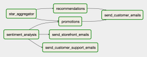
Screen Shot 2016-01-31 at 10.46.39 PM

This is a direct screen shot of a workflow from airflow. Similar to the Queue DAG, this flow of control looks a bit more complicated than a standalone monolithic program, so we’ll talk about what each piece does and why it’s designed this way.

To start, each node in the graph represents one distinct task, and each arrow implies a dependence on a previous item. For example, the ‘recommendations’ task is can’t run (is dependent) until the ‘star_aggregator’ task has completed.

Additionally, Each node in the DAG should be responsible for only one type of information or one task, and it should save the information either into a database or to disk in between each step. This differs slightly from the Queue DAG model, which required us to either transform or save information but not both. However, the queue itself acted as a data store in this case. Information posted for the next job was saved to the queue; essentially, we were relying on the queue to save data in between each step. For batch operations, we should do it ourselves.

The largest difference between the flow of control in batch systems vs queueing systems is that batch systems can set a dependency on more than one other task. In the above example, ‘send_customer_emails’ is dependent on both the ‘recommendations’ and ‘promotions’ task. Once both of those finish executing, we know we can execute the ‘send_customer_emails’ task. In a queue, there’s no way a node to determine if previous tasks have finished executing, only that there’s a unit of work available. In a batch system, we can keep track of which units of work have completed successfully, so we can have multiple dependencies in our system.


Benefits

Errors Cause Less Wasted Time

This is far and away the biggest reason why I’ve done things up like this in the past. It’s kind of inevitable. You’ve tested for all the cases currently in your database, but someone enters a control character that you didn’t think about, which causes your whole program to come crashing down around you. DAGs (and AirFlow particularly) help to keep you from losing too much time. When one task fails, all the tasks downstream don’t even bother to execute, so you can deploy a quick patch to your DAG, and only rerun the items that either failed or didn’t run because of a failure upstream. You don’t have to wait for your monolithic app to finish all the previous steps before executing your hot new fix.

Better Success State Handling

When a set of information is committed to the database in a monolithic app, you have no choice but to either say, ‘Everything completed successfully’ so as to not add duplicate data to the database or you have to do complex error handling states to determine if values have been successfully added or not. When using a DAG, each task is modularized so that an error at most points only requires rerunning the current node. The one exception to this is if the task fails midway through saving it to a data store, but any point leading up to that should be easy to fix, run again, and have correct output.

Minimizing Integration Points for Fast Debugging

In a monolithic app data structures can interact in ways that can lead to silent failures. An example of this may be that a method modifies 1,000 entries in your set early on in execution, no one realized what kind of issues this may lead to later on in execution, and now you have wrong data but don’t know how it got in there. This can be a nightmare to debug. In a DAG, we know the expected input, so diagnosing what led to this problem (such as an errant SQL call) becomes a routine case of opening your SQL client and trying out queries that will lead to the right answer.

Additionally, there are only so many places where each process can go wrong. The data loading, the transformation, and the saving. Right from the start, you know a task failed because of one of those things; not that something happened at the start of the program that was modified sixteen steps before the error was thrown in some nested function written by Steve at the end of the office. Walking the error back to the beginning of this particular process is a much, much shorter trip than going back thousands of lines of code in a monolithic ETL.

Better memory management

This is particularly true in languages that rely on garbage collection. Every C developer knows exactly where and when we should reclaim memory, but most of us aren’t C developers. In a monolithic app, a giant data structure that’s no longer used needs to be dereferenced in order for it to be eligible for garbage collection, so we’ve got to determine where and when every data structure is used and when it’s not being used anymore. Using a DAG model, the starting and stopping of tasks will implicitly handle this garbage collection for us. A massive set opened up for the first process in a long chain releases its memory as part of that task completing.

Cheap Multiprocess Support

This is especially true with Airflow’s simultaneous execution of many tasks. Let’s say we have an eight core EC2 instance. In monolithic apps, we’d have to pay very close attention to threading in our large scale processes; otherwise, we’re only using one of those cores. However, Airflow’s concurrency model will automatically run each non dependent process at the same time up to a certain limit (we don’t want our processors thrashing now). It will then run all the dependent processes concurrently as well. In the example above, ‘star_aggregator’ and ‘sentiment_analysis’ will run at the same time. After they’ve been completed successfully, ‘recommendations’, ‘promotions’, ‘send_storefront_emails’, and ‘send_customer_support_emails’ will be run simultaneously next. This has the net effect of significantly speeding up your execution time without putting in much more work.

Conclusion

For non-realtime processing, using a DAG model and a tool like Airbnb’s Airflow can significantly speed up your development time and make your code maintainable over the long haul. It’s can be slightly more work to define integration points and set up the dependencies, but those drawbacks are a one time investment for a system that will run better and smoother over the long haul.

Directed Acyclic Graphs (DAGs) for Queue Systems

Introduction

In the first part of this series, we discussed what a DAG is and what abstract benefits it can offer you. In this article, we’ll talk about its specific implementation in a queuing system. For this article, I’ll use customer reviews as an example; they’re relatively straightforward, but you’d be surprised at the steps that can occur when you rate your dog food five stars because Fluffy loved it.

This post assumes that the user is already familiar with Queues such as RabbitMQ or Kafka as well as worker threads that process these requests.

How to Implement a DAG

The Naive Way

It’s tempting to implement each worker as a one step process. You post a customer review to the queue, and a worker pulls it off, saves it to the database, sends off emails to the merchant, adds it to the star rating aggregation and then quits. I’ll explain why this is poor practice.

At what point do we define a success condition throughout this process? Do we say ‘mission accomplished’ only when the worker has finished all its tasks? Suppose it fails when it’s processing the aggregation. Now we have to rerun the entire worker process, which results in two entries in the database, two emails sent, but only one aggregate added to the database. We almost have to say ‘mission accomplished’ once its been added to the database to avoid duplication and mark it as ‘completed’ only when the worker has finished, but now we’re adding unnecessary state to the database and extra steps to the worker, steps that are a nightmare from a maintainability standpoint.


A Better Way

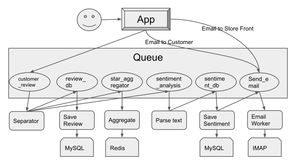
Screen Shot 2016-01-21 at 10.21.44 PM

I know this looks complicated, so bear with me for a moment, and I’ll explain what this is doing and why.

Each node in the DAG should either transform information or save it but not both. Why? There are a couple key reasons; some of which were covered in the first entry in the series, but we’ll look at those again as well as what’s specific to just the queue DAG.

Modularization

This is the most self-evident of the three big reasons. It’s easy to see in this case that the email node is being used by three wholly separate processes. The mail protocol isn’t likely to change from email to email, so as long as the information placed in the queue follows the same pattern, it’s trivial to reuse the same code. Additionally, it’s easy to imagine how a ‘storefront review’ form would map directly from the app to the sentiment analysis queue instead of the ‘customer_review’ queue.

Error Handling

This is easily the biggest of the top three. Since each node is only responsible for one task, there’s no work that gets redone as a result of a failure. If the sentiment analysis fails because of a flaw in the programming, we don’t need to care if it’s been saved successfully or if the star aggregator worked. We know that we can just try again when the code’s been fixed.

What makes this possible is that a queue worker only has to tell the queue that it successfully processed the message _after_ it’s finished. If there’s an error in the logic that prevents the successful completion of the task, it stays on the queue, and the worker tries again. Similarly, if there’s a network partition that keeps ‘Save Review’ from accessing the MySQL database, the message can go back on the queue to try again.

At the end of this article, I’ll list out the things you’ll want to save as error messages.

Scalability

This is the least thought about reason of the big three, but it’s also what gives this model a lot of power. The sentiment analysis here is the most CPU bound of all of the processes. Since any machine that has access can read from the queue, the workers for sentiment analysis can be placed on an Amazon C4XL for maximum power. The others are IO bound, so throw them on a micro instance, and you’ll be fine (don’t actually do that, but a small server would be totally fine).

Additionally, you can only process one queue at set intervals to save time and money. If you look at star ratings every hour but only review sentiment analysis first thing in the morning, then why not rent a machine for an hour each night to process the sentiment analysis queue? Or if you notice that no one does reviews at 2AM, start a cron job to only start sentiment analysis at 2AM on your smaller machine.

It’s Only Slightly More Work

Seriously. You were going to implement all the logic of the workers anyway, so why not take advantage of better architecture?

Error Messages

Since good error messages are the life blood of maintainability, this gets its own section.

In addition to placing information the next worker will need, the worker should also pass along these values to all subsequent workers; think of this as the queue stack trace. Here are the things you’ll want to save:

  • Worker name – Which worker threw the error (i.e. ‘Save Review’ above)
  • Time request was issued – What time did this worker first get the message?
  • Time request was finished – What time did this worker fail?
  • Processing time – How long was spent on this message? Did it churn for an hour or fail right away?
  • Status – Success or failure?
  • Server Name – IP Address or the name of the server this worker was running on
  • Message (maybe stack trace on error) – If you get a stack trace, put it in the error; this should go without saying :)
  • Queue Name – What queue did this worker pop off of
  • Queue Message Id – If operations are idempotent, list the message

Further reading:

If you want more theory and some more examples, one of the easiest to read is Queue-based System Architecture: Build Scalable, Fault-tolerant Distributed Systems. Added bonus: it’s free with Kindle Unlimited!

Directed Acyclyic Graphs (DAGs) for Non-Interactive Processing

Introduction

Since the introduction of the personal computer, interaction of users has become the default mode of developing applications, but as users come to expect more and more features with less and less processing time. If Amazon generated a new recommendation list on each page load, they wouldn’t have gotten very far in the retail space.

Explanation of Terms

That title’s a mouthful, so let’s break down some of the terms and how they relate to each other.

Non-Interactive Processing

Non-Interactive Processing is any type of information processing where the user doesn’t expect immediate feedback for their actions. Typically most things we associate with user applications are interactive processing. When you update your status on Facebook, you expect to be notified of its status. When you click ‘Purchase’ on your Amazon mobile app, you expect to be notified of an issue with your credit card immediately. Non-Interactive processing is anything that is pushed off to be processed later. Your Amazon recommendations are a great example of this.

Directed Acyclic Graphs

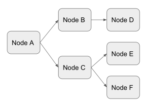
A graph is a mathematical structure that has any combination of nodes and edges linking those nodes (seen below)

Screen Shot 2016-01-18 at 7.33.20 PM

In software engineering, and for the purposes of this blog, we say that nodes represent a collection of statements that the machine will execute and the edges represent a transition from one collection of commands to another.

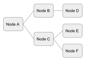
A directed graph is a graph in which one node has a directional transition from one node to another (see below)

Screen Shot 2016-01-18 at 7.34.03 PM

In this example, Node A can transition to Node B and Node B can transicion to D, but Node B can never transition back to Node A. In a standard directed graph, the nodes could be organized so that B points back to A as well, which brings us to the idea of an Directed Acyclic Graph (DAG). An Acyclic Graph requires that no node be able to execute twice. In other words, once a Node has finished running, there should be no way for it to be able to run again. The above graph is acyclic, and below are some examples of graphs that are not acyclic.


In example 1, A->B->A. In example 2, A->B->D->A. In example 3, A->B->D->E->F->A. All of these are examples of graphs where cycles exist (non-acyclic)


Putting it back together

One of the most common ways in which non-interactive programs are structured is using DAGs. Some of this is historical. Unix systems, for example, come with a wide selection of commands that do one small task very well, and the results of these tasks are then forwarded to other tasks. As we’ll see in the rest of this post (as well as future ones), setting up your non-interactive systems using DAGs is just good design as well.


Benefits

Modularization

Each node in the DAG is responsible for one task and one task only. Not only does this help us sort out responsibility in an effective way, but it also means that we can reuse any component in multiple DAGs.

For example, Twitter email you several times a week about tweets in your network and people you should be following. This module can now be reused to email you when you’ve been retweeted.

The argument could be made to export the email function as a library and use the library instead, but we’ll see in later entries about (!!!) and (!!!) that separating them can have very useful, even necessary consequences.

Not Repeating Work

This especially holds true for batching systems, but one monolithic ETL app that processes all your information from start to finish can be very expensive when the system fails. Imagine a batching system that runs for 20 hours, and it fails at hour 19. If it’s one monolithic app, you need to repeat those 19 hours to get to the last hour that failed to run. When you divide the work into self-contained, modularized nodes, you only need to repeat that last hour once the bugs have been fixed.

Stitching Together Languages

Every language does one particular thing very, very well. For example, I’m a big fan of MySQL’s Java library for batch inserts, but Python handles statistical data manipulation sooooo much better. One of my favorite tricks is to do all your statistical processing in Python, flush the data to disk as a CSV, and have Java read them in and batch insert everything. It sounds complicated, but, since you’ve modularized the Python and Java code, stitching them together with a DAG is easier and quicker than using one language to do both things.

Moving Forward

Now that we’ve got the basics covered, we’ll move into two implementations of the DAG, queueing systems and batch processing (forthcoming).